How to Find Matching Values in Two Columns in Excel

Excel has a special talent: it can turn “I just need to compare two lists” into a three-hour existential crisis. The good news? Finding matching values in two columns is one of those skills that feels like magic once you know a few reliable moves. The better news? You don’t need magicjust the right tool for the job.

In this guide, you’ll learn multiple ways to find matches between two columns in Excelfrom quick visual highlighting to formulas (including modern dynamic arrays) to Power Query for big, messy datasets. Along the way, we’ll cover common “gotchas” like extra spaces, text-vs-number mismatches, and duplicates that refuse to behave.

First, decide what “matching” actually means

Before you pick a method, answer one question: what kind of match do you need? Excel can do several different “matching” jobs, and choosing the wrong one is like bringing a spoon to a pizza party.

• Exists anywhere in the other column: “Does A2 appear anywhere in column B?” (Great for comparing two lists.)
• Matches in the same row: “Does A2 equal B2?” (Great for row-by-row validation.)
• Return related info: “If A2 matches something in column B, return a value from column C.” (Classic lookup use case.)
• Extract a clean list of matches: “Give me a new list containing only the items that appear in both columns.” (Perfect for reporting.)

Method 1: Highlight matches visually (Conditional Formatting)

If your goal is to spot matches quickly (not build a reusable result), Conditional Formatting is the fastest win. It’s also the least likely to start a formula war in your workbook.

Option A: Built-in “Duplicate Values” rule (quickest)

1. Select both columns you want to compare (for example, A:A and B:B, or a smaller range like A2:B200).
2. Go to Home > Conditional Formatting > Highlight Cells Rules > Duplicate Values.
3. Pick a format color and click OK.

Excel treats duplicates across the selected range as matchesso values appearing in both columns will be highlighted. This is perfect for quick audits, but it’s not “logic-aware” (it highlights duplicates within a single column too).

Option B: A custom rule to highlight only “A in B” matches

Want Excel to highlight only the values in column A that exist somewhere in column B? Use a formula rule:

1. Select the range in column A you want to format (example: A2:A200).
2. Go to Home > Conditional Formatting > New Rule.
3. Choose Use a formula to determine which cells to format.
4. Enter this formula:

Click Format, choose a highlight style, and save. Now column A lights up only when its value exists in column B. Repeat the idea the other direction if you want B-in-A highlighting too.

Method 2: Use formulas to mark matches (reliable and reusable)

Formulas are the go-to choice when you want results that update automatically as data changes. Below are several formula patternspick the one that fits your situation.

2.1 The simplest “does it exist?” check: COUNTIF

If you just want a yes/no match flag next to your values:

Copy it down next to your list in column A. This checks whether A2 appears anywhere in column B. If you don’t need words, you can return TRUE/FALSE instead:

Tip: COUNTIF is forgiving and fast for many everyday lists. It’s also easy to read later (future-you will appreciate it).

2.2 A classic match test: ISNUMBER(MATCH())

MATCH finds the position of a value within a range. If it’s found, MATCH returns a number (the position); if not, it returns an error. Wrap it with ISNUMBER to convert “found/not found” into TRUE/FALSE:

If you prefer readable text:

Why people like this: It’s a well-known pattern, widely supported, and works nicely in conditional formatting rules.

2.3 The modern version: XMATCH (Microsoft 365 / newer Excel)

If you have XMATCH, it’s a cleaner MATCH cousin:

XMATCH can be more flexible than MATCH in advanced scenarios, but for basic “exists” checks, both work great.

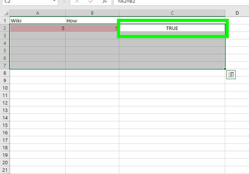
2.4 Match in the same row (A2 vs B2)

Sometimes you’re not comparing two listsyou’re validating two columns that should line up row-by-row (like “Expected ID” vs “Actual ID”). Then you want a direct comparison:

For a friendly label:

Case-sensitive? Use EXACT:

Method 3: Return related data when a match is found (lookups)

If you need more than “Match/No match”for example, “If this email exists in the master list, return the customer tier” then you want a lookup function.

3.1 XLOOKUP (best all-around if you have it)

XLOOKUP can search one column and return a related value from another columnwithout the classic VLOOKUP limitations. Example: You have IDs in column A, and a reference table in columns D (ID) and E (Status). Return the status:

If you want to return the matching value itself (instead of related data), just set the return array to the same lookup array:

3.2 VLOOKUP (still useful, but know its quirks)

VLOOKUP is common in older workbooks and still works fineespecially for straightforward tables. The key thing to remember: it looks in the leftmost column of your table and returns a value to the right.

The last argument matters: FALSE means exact match. If you use TRUE (or omit it), Excel may do an approximate match, which is a great way to accidentally “match” the wrong thing with confidence.

3.3 INDEX + MATCH (solid and flexible)

If you’re in a workbook where INDEX/MATCH is the house style, this combo is still excellent:

It’s flexible (can look left, right, up, down) and doesn’t break as easily if columns are inserted into your table.

Method 4: Extract a list of matching values (dynamic arrays)

If you have Excel for Microsoft 365 (or a version with dynamic arrays), you can generate a clean list of matches without helper columns. This is chef’s-kiss-level Excel.

4.1 FILTER + COUNTIF: pull matches from list A that appear in list B

Suppose list A is A2:A100 and list B is B2:B100. To extract the values from A that appear in B:

Want a unique list (no repeats) of matching values? Wrap with UNIQUE:

This is especially handy when you’re building a report tab and don’t want to babysit it every time new rows are added.

Method 5: Power Query (best for large, messy, repeatable comparisons)

If you’re comparing thousands (or hundreds of thousands) of rows, or you need a process you can repeat weekly with new files, Power Query is the grown-up solution. Think of it as Excel’s data-prep kitchen: you bring the ingredients; it does the chopping.

Use “Merge” to join tables by matching values

The core idea is simple: load both lists as queries, then merge them on the key column. You can choose different join types depending on what you want:

• Inner join: returns only matches (items that appear in both).
• Left outer: keeps all from the first list and shows matches from the second (great for finding missing items).
• Anti-joins: returns only non-matches (pure “what’s missing?” lists).

High-level steps (no tears required)

1. Convert each list into a Table: select data, then press Ctrl + T.
2. Go to Data > From Table/Range to load each table into Power Query.
3. In Power Query, choose Home > Merge Queries (or “Merge Queries as New”).
4. Select your matching column in both tables (for example, “CustomerID”).
5. Pick a join type (Inner for matches-only is usually the starting point).
6. Expand the merged column to show details or keep it as a match indicator.
7. Close & Load back to Excel.

Power Query shines when your data changes often, comes from exports, or contains “Excel crime scenes” like inconsistent formatting. Once built, a query can be refreshed with one click.

Clean your data first (because Excel matches exactlyeven when humans don’t)

Many “no match” results are actually “your data is wearing a disguise” results. Here are the most common culprits:

Extra spaces

A trailing space makes “ABC123” not equal to “ABC123 ”. Use TRIM to remove extra spaces:

Invisible characters

Data copied from websites or systems sometimes includes non-printing characters. CLEAN helps:

Numbers stored as text

“1001” (text) may not match 1001 (number) depending on context. You can normalize with VALUE:

Case sensitivity

Most matching methods are case-insensitive (“abc” matches “ABC”). If you need case-sensitive matching, use EXACT.

Partial matches and “close enough” searching

Sometimes you don’t want an exact match. Maybe column A contains “Acme Corp – West” and column B contains “Acme Corp.” That’s where SEARCH (or wildcards) comes in.

Check if a cell contains a substring

This returns TRUE if the text in B2 appears anywhere inside A2 (case-insensitive). For case-sensitive substring checks, use FIND instead of SEARCH.

Wildcard matching with lookups

Some workflows use wildcards like * (any characters) or ? (single character). Example pattern: find a value that starts with “ACME”:

Use partial matching carefullyit’s easy to match “Ann” inside “Joann” and then spend the afternoon investigating a phantom customer.

Troubleshooting: when matches “should” work but don’t

• You’re getting #N/A: That usually means “not found.” Add an “if not found” argument in XLOOKUP or wrap legacy formulas with IFERROR:
• Duplicates are confusing the result: If a value appears multiple times in the lookup list, XLOOKUP/VLOOKUP typically returns the first match. If you need all matches, use FILTER (dynamic arrays) or Power Query.
• Performance is slow: Full-column references ($A:$A) are convenient but can be heavy in huge files. Use realistic ranges (like A2:A50000) or Excel Tables with structured references.
• Approximate match mistakes: For VLOOKUP, remember that TRUE/omitted can return “nearest” results. Use FALSE for exact matches unless you truly want approximate behavior.

Wrap-up: the best method depends on your goal

If you want quick visuals, Conditional Formatting is fast and friendly. If you need a reusable yes/no result, COUNTIF or ISNUMBER(MATCH()) is dependable. If you’re pulling related values, XLOOKUP is the modern favorite (with VLOOKUP and INDEX/MATCH still useful in many workbooks). And if your data is big, messy, or recurring, Power Query is the long-term sanity saver.

Real-world “Excel trench” experiences (common scenarios + lessons learned)

Below are the kinds of situations where people use two-column matching in the wildplus what usually goes wrong, and how to avoid the classic mistakes. These aren’t fairy tales. They’re the spreadsheet equivalent of “based on a true story,” minus the dramatic soundtrack (unless you count keyboard clacking).

1) “Why don’t these customer IDs match? They LOOK identical.”

This is the #1 reality check: humans see “same,” Excel sees “not even close.” Most of the time, the culprit is invisible: extra spaces, non-printing characters, or numbers stored as text. The fix is almost always a quick normalization step. A surprisingly effective approach is to add helper columns with: TRIM for spaces, CLEAN for weird characters, and VALUE (or multiplying by 1) to coerce text-numbers into real numbers. Once both sides are “speaking the same data language,” your MATCH or COUNTIF suddenly starts behaving like a functional adult.

2) Email lists: “We emailed 12,000 people. Who didn’t get it?”

Email comparison sounds simple until you remember that email addresses come with bonus chaos: capitalization differences, leading/trailing spaces, and occasional “invisible” issues from copy/paste. A practical workflow is: normalize emails to lowercase (so “[email protected]” matches “[email protected]”), trim spaces, then use COUNTIF or XMATCH to flag which campaign list entries exist in the master CRM list. If you need the actual “missing” list, FILTER is perfect: it can spill a clean list of “not found” addresses to hand off for follow-upno manual sorting and praying required.

3) Inventory and SKUs: “Same product, different system, different naming.”

Matching SKUs is where partial matches tempt you like a shortcut with a speed trap. If one system stores “ACME-1001-BLACK” and another stores “1001” or “ACME 1001,” exact matches will fail. People often reach for wildcards or SEARCH-based checks. That can work, but it can also create false positives (like matching “100” inside “1000”). The safer approach is to extract a consistent keymaybe the numeric portion or a standardized codeinto helper columns using text functions, then match the standardized keys exactly. When this becomes a monthly ritual with new exports, Power Query is the hero: you can split columns, clean values, and merge tables the same way every refresh.

4) Finance reconciliation: “These payments should match… somewhere.”

Reconciliation often starts with “Does this transaction ID exist in the bank export?” but ends with “Why are there duplicates and reversals and corrections and… oh no.” Here, the big lesson is: define the match criteria clearly. Sometimes you match on ID only; other times you match on multiple fields (ID + date + amount). In formula-land, that can mean COUNTIFS across multiple columns. In Power Query, it means merging on multiple keys. The win is huge: once you build a repeatable comparison, your “recon day” goes from frantic detective novel to mildly boring checklistwhich is the best kind of boring.

5) HR or training compliance: “Who’s on the roster but not on the completion list?”

This is a classic two-list comparison: employee roster vs completion list. A clean pattern is: use a “Match?” helper column with ISNUMBER(XMATCH()), then filter to show only FALSE values. For leaders who want a crisp answer, you can produce a spilled list of missing names with FILTER. The biggest practical mistake here is inconsistent naming (middle initials, suffixes, nicknames). The real fix is using a unique identifier (employee ID) whenever possible. Names are for humans; IDs are for Excel.

The overall takeaway from these scenarios is simple: most matching problems aren’t “Excel problems”they’re data definition problems. Once you decide what “match” means, clean the data so it’s comparable, and choose the method that fits the size and frequency of the task, Excel becomes less of a chaos gremlin and more of a helpful assistant. (Still slightly smug. But helpful.)

SEO tags (JSON)