

Missed Prime Day? You may still have time to save. This guide rounds up 50 extended Amazon...
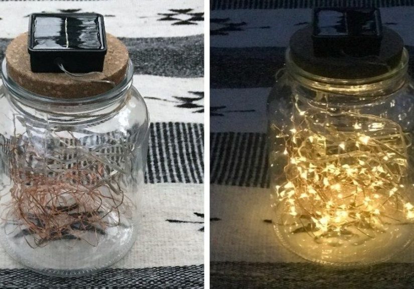
Turn an ordinary glass jar into a glowing little galaxy with this simple guide to making a...
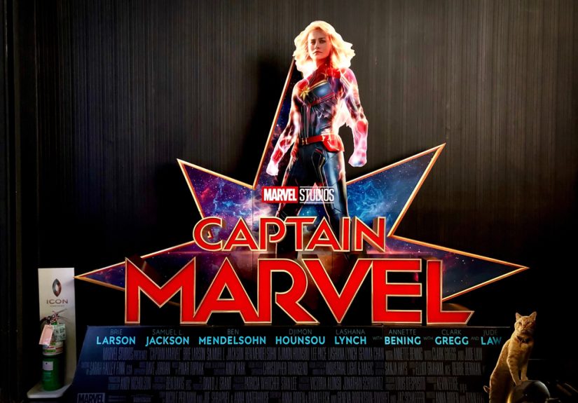
Superhero movies are not just capes, cosmic battles, and cities with terrible insurance premiums. From the perspective...
Looking for a beautiful Christmas tree without the mess, watering, or yearly price shock? Walmart’s faux Christmas...

Abuse can be confusing, isolating, and emotionally exhausting, but you do not have to face it alone....

Winter photos have a special power: they turn snow, lights, cozy rooms, and small seasonal details into...

Gout and turf toe can both make the big toe swollen, painful, stiff, and difficult to walk...
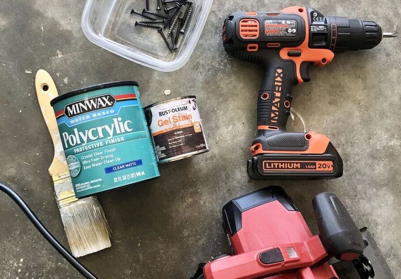
Wire shelves are practical, but they can also be wobbly, messy, and frustrating when small items tip...

Women now make up the majority of U.S. medical students, but leadership in medicine still tells a...